More about Cell Complexes

An excellent simple introduction to the area of DCCs with their various applications is given in the book of Leo Grady and Jonathan Polimeni Discrete Calculus. Applied Analysis on Graphs for Computational Science. (2010) Below are just a few notes necessary for understanding the output of the code.

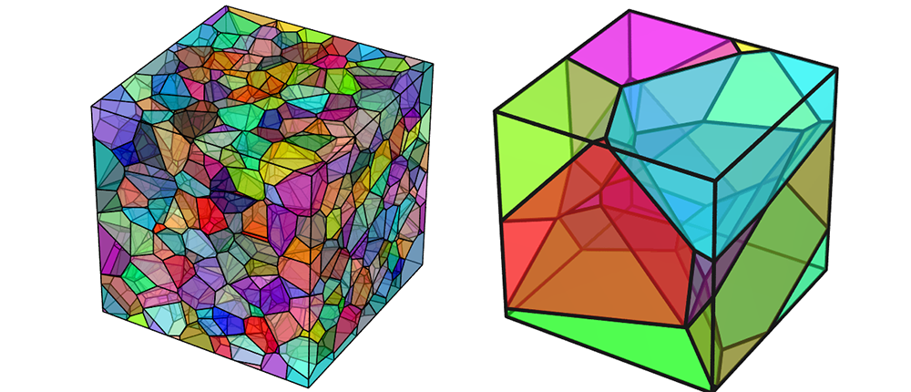
• In algebraic topology, a discrete topological n-complex is a collection of cells of dimensions k ≤ n , where every k-cell for any 0 < k ≤ n has a boundary formed by (k-1)-cells belonging to the complex. The co-boundary of every k-cell for 0 ≤ k < n is the set of (k+1)-cells whose boundaries contain the k-cell. In this terminology, 1-complex is a graph. Polyhedral complexes are a special class of regular quasi-convex discrete topological complexes, in the geometric realisation of which 0-cells are identified with points or vertices, 1-cells with line segments or edges, 2-cells with planar polygons or faces, 3-cells with polyhedra or simply cells, etc. We restrict our consideration to the polyhedral 3-complexes whose 3-cells are convex polyhedra with 2-cells in the boundary of exactly two 3-cells. An assembly of polyhedrons is a geometric realisation of a combinatorial structure referred to as a cell complex in algebraic topology.
• The geometric properties of the DCC are encoded in the volumes of different cells: 1 for 0-cells, length for 1-cells, area for 2-cells, and volume for 3-cells. The topological properties of the DCC are encoded in the boundary operator B_k, which maps all (k+1)-cells to the k-cells in their boundaries, taking into account cell orientations. The algebraic realisation of the operator for the [k,(k+1)] pair of cells is referred to as the k-th incidence matrix, B_k, which has N_k rows (where N_k denote the number of k-cells in a complex) and N_k+1 columns and contains 0, 1, -1, indicating non-adjacency, adjacency with agreeing and with opposite orientations, respectively, between k-cells and (k+1)-cells. The transpose of the k-th incidence matrix, b_k = B_k^T, is a matrix representing the k-th co-boundary operator, which maps all k-cells to the (k+1)-cells in their co-boundaries.
• A standard way is to decide on a consistent orientation of all top-dimensional cells, e.g., to select the positive orientation to be from interior to exterior of the 3-cells and assign arbitrary orientations for all lower-dimensional cells. There are exactly three options for the relation between k-cell and (k+1)-cell in an oriented complex: they are not coincident - encoded by 0; the k-cell is on the boundary (k+1)-cell, and they have consistent orientations, encoded by 1; the k-cell is on the boundary (k+1)-cell and they have opposite orientations, encoded by -1. The transpose of the k-th incidence matrix is a matrix representing the k-th co-boundary operator, which maps all k-cells to the (k+1)-cells in their co-boundaries.
• The k-th combinatorial Laplacian (Laplace–de Rham operator) can be written as
  L_k = b_k-1 B_k-1 + B_k b_k
  and it maps all k-cells to themselves, collecting local connectivity information. One important application of the combinatorial Laplacians is in calculating combinatorial curvatures . Since the Laplacians are symmetric positive semi-definite matrices, their eigenvalues are real. The spectra of eigenvalues can be used to classify discrete topologies, with two topologies considered equivalent when they have the same Laplacians’ spectra.